Generalized least squares

Find the GLS estimate and the variance of its components in the case where the error covariance matrix $V_{n}$ is diagonal.

Obtain a matrix of the form (11.12).

Let $X_{k} = \theta_{1}+\theta_{2} h_{k}+\varepsilon_{k}, k = 1,2,3$, where the error vector $E = \left\{ \varepsilon_{1}, \varepsilon_{2}, \varepsilon_{3}\right\}^{T}$ has expectation $\mathbb {E}\left[E\right] = 0$, and $\operatorname {Cov}\left[ E, E \right] = \sigma^{2} V$,

the numbers $a$ and $0 < \rho < 1$ are unknown, $h_{1} = -1, h_{2} = 0, h_{3} = 1$. Show that the GLS estimate of the vector $\theta$ has the form

where $r = 1+\rho +2 a^{2}-4 a \rho$. Find values of $\rho , a, X_{k}, k = 1,2,3$ for which the regression line lies entirely below all the observed values, and values for which it lies entirely above them.

Let $X_{i} = \theta h_{i}+\varepsilon_{i}, i = 1,2$, where $\varepsilon_{1} \sim \mathcal{N}\left(0, \sigma^{2}\right), \varepsilon_{2} \sim \mathcal{N}\left(0,4 \sigma^{2}\right)$, and $\varepsilon_{1}$ and $\varepsilon_{2}$ are independent. For two vectors $h: h^{(1)} = [-1,1]^{\top }, h^{(2)} = [1,-1]^{\top }$ find the GLS estimate and its variance for the two vectors $h$.

Let the regression model have the form

where $\varepsilon_{k}$ are independent centered random variables with variances $\sigma_{k}^{2} = h_{k}^{2}$. From the observations given in Table 11.5, find the realizations of the OLS estimate and the GLS estimate of the unknown parameters $\left[\theta_{1}, \theta_{2}\right]^{\top }$. For each estimate, compute the covariance matrix of its error.

Table 11.5

Show that applying GLS to the simple linear regression model with error variances equal to $\operatorname {Var}\left[e_{k}\right] = \sigma^{2} h_{k}^{2}$ is equivalent to applying ordinary least squares to the observation model of the form

where $\delta_{k}$ are independent random variables with variances $\operatorname {Var}\left[\delta_{k}\right] = \sigma^{2}$ for $k = 1, \ldots , n$.

Consider the regression model

where the errors $\varepsilon_{k}$ satisfy the first-order autoregression equation

where $v_{k}$ is a sequence of independent normally distributed random variables with zero mean and variance $\sigma_{0}^{2} = 1$. Find the realization of the GLS estimate of the vector of unknown parameters $\theta = \left[\theta_{1}, \theta_{2}\right]^{\top }$ from the observations given in Table 11.6.

Table 11.6

Compare the obtained vector with the realization of the OLS estimate constructed under the assumption that the errors $\varepsilon_{k}$ are uncorrelated.

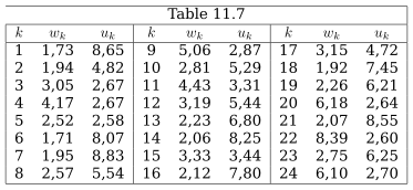
Consider the model relating the number of vacancies $w$ and the unemployment rate $u$

where $X_{k} = \ln w_{k}, h_{k} = \ln u_{k}, \varepsilon_{k} \sim \mathcal{N}\left(0 ; \sigma^{2}\right)$. Using the data from Table 11.7, find the OLS estimates of the parameters $\theta_{1}$ and $\theta_{2}$. Use the Durbin-Watson test to test the hypothesis $H_{0}: \rho = 0$ that the observation errors are uncorrelated, at the significance level $\alpha = 0,05$. If the hypothesis $H_{0}$ is rejected, assume that the sequence of random errors $\left\{ \varepsilon_{k}\right\}$ satisfies the first-order autoregression equation

where $e_{k}$ are centered Gaussian random variables with variance $\operatorname {Var}\left[e_{k}\right] = \sigma_{0}^{2}$. Find an estimate of the unknown coefficient $\rho$ in the autoregression equation.

Investigate the consumption function of Japan $X(h)$ over the period 1951-1962 for correlation of the observation errors. If the observation errors are correlated, find the realization of the GLS estimate of the vector of unknown parameters. Find an estimate of the covariance matrix of the error vector $E$. The data for the computations are given in Table 11.8 (data taken from: U. N. Yearbook of National Accounts Statistics, 1963). Here $X$ is aggregate individual consumption (trillion yen), and $h$ is aggregate personal income (trillion yen).

Table 11.8

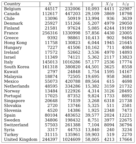
Investigate the dependence between manufacturing value added ($X$) and gross domestic product ($h$) on a sample of 28 countries for 1994 that includes both small and large countries (UNIDO Yearbook 1997). Table 12.5 gives the values of $X$ and $h$ in millions of US dollars, the population $(g)$ in millions of people, and the data in the last two columns in US dollars per person. Construct the OLS estimate of the parameters $\theta_{1}$ and $\theta_{2}$ for the model

Check for heteroscedasticity using one of the tests, assuming that the observation errors $\varepsilon_{k}, k = 1, \ldots , 28$ are uncorrelated and Gaussian. If heteroscedasticity is detected, eliminate it by dividing each observation by the population value. For this, the data from the last two columns of Table 12.5 can be used.

Table 12.5

The weighing of three loads with masses $a$ and $b$ is carried out as follows: the first load is weighed $n_{1}$ times (all measurement errors have distribution $\mathscr {N}\left(0, \sigma^{2}\right))$, the second load is weighed $n_{2}$ times on the same scale, then the first and second loads together are weighed $n_{3}$ times on a different scale, whose measurement errors all have distribution $\mathscr {N}\left(0, 3 \sigma^{2}\right)$. Reduce the problem to a linear model and find the least-squares estimators for $a$ and $b$, as well as the optimal estimator for $\sigma^{2}$.

Let the vector $X=\left(X_{1}, \ldots , X_{n}\right)$ have distribution $\left(a b, \sigma^{2} \Sigma \right)$, where $b$ is a known vector of dimension $n$, $\Sigma$ is a known positive-definite matrix, and $a$ and $\sigma^{2}$ are unknown parameters. Reduce the problem to a linear Gaussian model and find the least-squares estimators of the parameters $a$ and $\sigma^{2}$.

Let $X_{i} \sim N\left(a, i \sigma^{2}\right), i=0,1, \ldots , n, Y_{i} \sim \mathscr {N}\left(jb, \sigma^{2}\right), j=1, \ldots , m$ be independent random variables, where $a, b, \sigma^{2}$ are unknown parameters. Reduce the problem to a linear model and construct an $F$-test of size $\alpha$ for testing the hypothesis $H_{0}: a+b=1$.

Let $Y_{i} = \beta x_{i}+\varepsilon_{i}(i = 1,2)$, where $\varepsilon_{1} \sim N\left(0, \sigma^{2}\right), \varepsilon_{2} \sim N\left(0,2 \sigma^{2}\right)$, and $\varepsilon_{1}$ and $\varepsilon_{2}$ are statistically independent. If $x_{1} = +1$ and $x_{2} = -1$, obtain the weighted least squares estimate of $\beta$ and find the variance of your estimate.

Let $Y_{i}(i = 1,2, \ldots , n)$ be independent random variables with a common mean $\theta$ and variances $\sigma^{2} / w_{i}(i = 1,2, \ldots , n)$. Find the linear unbiased estimate of $\theta$ with minimum variance, and find this minimum variance.

Let $Y_{1}, Y_{2}, \ldots , Y_{n}$ be independent random variables, and let $Y_{i}$ have a $N\left(i \theta , i^{2} \sigma^{2}\right)$ distribution for $i = 1,2, \ldots , n$. Find the weighted least squares estimate of $\theta$ and prove that its variance is $\sigma^{2} / n$.

Let $Y_{1}, Y_{2}, \ldots , Y_{n}$ be random variables with common mean $\theta$ and with dispersion matrix $\sigma^{2} \mathbf{V}$, where $v_{i i} = 1(i = 1,2, \ldots , n)$ and $v_{i j} = \rho$ ($0 < \rho < 1 ; i, j = 1,2, \ldots , n ; i \neq j$). Find the generalized least squares estimate of $\theta$ and show that it is the same as the ordinary least squares estimate. Hint: $\mathbf{V}^{-1}$ takes the same form as $\mathbf{V}$.

Let $\mathbf{Y} \sim N_{n}\left(\mathbf{X} \beta , \sigma^{2} \mathbf{V}\right)$, where $\mathbf{X}$ is $n \times p$ of $\operatorname {rank} p$ and $\mathbf{V}$ is a known positive-definite $n \times n$ matrix. If $\beta^{*}$ is the generalized least squares estimate of $\mathbf{\beta }$, prove that

Suppose that $\mathbb {E}\left[\mathbf{Y}\right] = \mathbf{\theta }, \mathbf{A} \mathbf{\theta } = \mathbf{0}$, and $\operatorname {Var}\left[\mathbf{Y}\right] = \sigma^{2} \mathbf{V}$, where $\mathbf{A}$ is a $q \times n$ matrix of $\operatorname {rank} q$ and $\mathbf{V}$ is a known $n \times n$ positive-definite matrix. Let $\mathbf{\theta }^{*}$ be the generalized least squares estimate of $\mathbf{\theta }$; that is, $\mathbf{\theta }^{*}$ minimizes $(\mathbf{Y}-\mathbf{\theta })^{T} \mathbf{V}^{-1}(\mathbf{Y}-\mathbf{\theta })$ subject to $\mathbf{A} \mathbf{\theta } = \mathbf{0}$. Show that

where $\tilde{\mathbf{\gamma }}^{*}$ is the generalized least squares estimate of $\mathbf{\gamma }$ for the model $\mathbb {E}\left[\mathbf{Y}\right] = \mathbf{V A}^{T} \mathbf{\gamma }, \operatorname {Var}\left[\mathbf{Y}\right] = \sigma^{2} \mathbf{V}$.

Let $Y_{1}, Y_{2}, \ldots , Y_{n}$ be independent random variables such that for $i = 1,2, \ldots , n$,

and

Given the regression line

where the $\varepsilon_{i}$ are independent with $\mathbb {E}\left[\varepsilon_{i}\right] = 0$ and $\operatorname {Var}\left[\varepsilon_{i}\right] = \sigma^{2} x_{i}^{2}$, show that weighted least squares estimation is equivalent to ordinary least squares estimation for the model

If the first column of $\mathbf{X}$ is $\mathbf{1}_{n}$ and

use (9.8) to show that

Hint: Consider $\mathbf{P 1}_{n}$.

When $\operatorname {Var}\left[\varepsilon \right] = \sigma^{2} \mathbf{V}$, the appropriate estimate of $\mathbf{\beta }$ is the generalized least squares estimate $\beta * = \left(\mathbf{X}^{T} \mathbf{V}^{-1} \mathbf{X}\right)^{-1} \mathbf{X}^{T} \mathbf{V}^{-1} \mathbf{Y}$. If $\mathcal{C}\left(\mathbf{V}^{-1} \mathbf{X}\right) = \mathcal{C}(\mathbf{X})$, show that $\mathbf{\beta }^{*}$ and $\widehat{\mathbf{\beta }}$ are identical. Hint: $\mathbf{V}^{-1} \mathbf{X} = \mathbf{X W}$, where $\mathbf{W}$ is nonsingular.

An experimenter wishes to estimate the density $d$ of a liquid by weighing known volumes of the liquid. Let $Y_{i}$ be the weight for volume $x_{i}(i = 1,2, \ldots , n)$ and let $\mathbb {E}\left[Y_{i}\right] = d x_{i}$ and $\operatorname {Var}\left[Y_{i}\right] = \sigma^{2} f\left(x_{i}\right)$. Find the least squares estimate of $d$ for the following cases:

Let $Y_{i} = \beta_{0}+\beta_{1} x_{i}+\varepsilon_{i}(i = 1,2,3)$, where $\mathbb {E}\left[\varepsilon \right] = 0, \operatorname {Var}\left[\varepsilon \right] = \sigma^{2} \mathrm{~ V}$ with

and $x_{1} = -1, x_{2} = 0$, and $x_{3} = 1$. Show that the generalized least squares estimates of $\beta_{0}$ and $\beta_{1}$ are

where $r = 1+\rho +2 a^{2}-4 a \rho$. Also prove the following:

If $\mathbf{X}$ is not of full rank, show that any solution $\mathbf{\beta }$ of $\mathbf{X}^{T} \mathbf{V}^{-1} \mathbf{X} \mathbf{\beta } = \mathbf{X}^{T} \mathbf{V}^{-1} \mathbf{Y}$ minimizes $(\mathbf{Y}-\mathbf{X} \mathbf{\beta })^{T} \mathbf{V}^{-1}(\mathbf{Y}-\mathbf{X} \mathbf{\beta })$.

Let $Y_{i} = \beta x_{i}+u_{i}, x_{i} > 0(i = 1,2, \ldots , n)$, where $u_{i} = \rho u_{i-1}+\varepsilon_{i}$ and the $\varepsilon_{i}$ are independently distributed as $N\left(0, \sigma^{2}\right)$. If $\widehat{\beta }$ is the ordinary least squares estimate of $\beta$, prove that $\operatorname {Var}\left[\widehat{\beta }\right]$ is inflated when $\rho > 0$.

Suppose that

where $\rho \in \mathbb {R}$ is an unknown parameter, $t_i$'s are known and in $(a,b)$, $a$ and $b$ are known positive constants, and $\varepsilon_i$'s are independent random variables satisfying $\mathbb {E}\left[\varepsilon_i\right]=0$, $\mathbb {E}\left[\left|\varepsilon_i\right|^{2+\delta }\right]<\infty$ for some $\delta >0$, and $\operatorname {Var}\left[\varepsilon_i\right]=\sigma^2t_i$ with an unknown $\sigma^2>0$.

1. Obtain the LSE of $\rho$.

2. Obtain the BLUE of $\rho$.

3. Show that both the LSE and BLUE are asymptotically normal and obtain the asymptotic relative efficiency of the BLUE with respect to the LSE.

References

[ГПП12] Горяинова Е.Р., Панков А.Р., Платонов Е.Н. Прикладные методы анализа статистических данных. Издательский дом Высшей школы экономики, 2012.
[ЖРШ16] Жуковский М.Е., Родионов И.В., Шабанов Д.А. Введение в математическую статистику. МФТИ, 2016.
[SeLe03] Seber G.A., Lee A.J. Linear Regression Analysis. 2nd ed., John Wiley & Sons, 2003.
[Sha05] Shao J. Mathematical Statistics: Exercises and Solutions. Springer, 2005.