Heteroscedasticity

Table 12.4 gives data on investment ($X$), government expenditure $\left(h_{1}\right)$, gross domestic product ($h_{2}$) and population $\left(h_{3}\right)$ for 28 countries in 1997. The quantities $X, h_{1}$ and $h_{2}$ are given in billions of US dollars, and $h_{3}$ in millions of people. Construct a dependence of the volume of investment on the volume of government expenditure and GDP of the form

where $\theta_{1}, \ldots , \theta_{4}$ are unknown parameters and $\varepsilon_{k} \sim \mathcal{N}\left(0 ; \sigma_{k}^{2}\right)$. Test the hypothesis $H_{0}: \sigma_{1}^{2} = \sigma_{2}^{2} = \cdots = \sigma_{28}^{2}$ using the Goldfeld-Quandt test at the significance level 0,05.

Table 12.4

Apply Bartlett's test to the data of Problem 1.

For the data of Problem 1, construct the dependence of investment on government expenditure and gross domestic product, dividing the values of all variables by the corresponding population value. Apply the Goldfeld-Quandt test to the new set of observations.

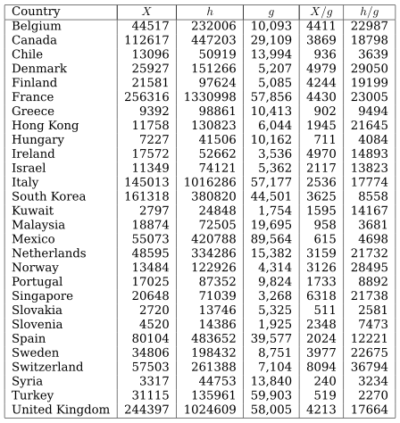
Investigate the dependence between manufacturing value added ($X$) and gross domestic product ($h$) on a sample of 28 countries for 1994 that includes both small and large countries (UNIDO Yearbook 1997). Table 12.5 gives the values of $X$ and $h$ in millions of US dollars, the population $(g)$ in millions of people, and the data in the last two columns in US dollars per person. Construct the OLS estimate of the parameters $\theta_{1}$ and $\theta_{2}$ for the model

Check for heteroscedasticity using one of the tests, assuming that the observation errors $\varepsilon_{k}, k = 1, \ldots , 28$ are uncorrelated and Gaussian. If heteroscedasticity is detected, eliminate it by dividing each observation by the population value. For this, the data from the last two columns of Table 12.5 can be used.

Table 12.5

Using a sample of 15 countries, estimate the parameters of the model $X = \theta_{1} + \theta_{2} h_{2}+\theta_{3} h_{3}$, where $X$ is per capita income; $h_{2}$ is the percentage of the labor force employed in agriculture; $h_{3}$ is the average level of education of persons over 25 years of age (the number of years spent in educational institutions). Test for the presence or absence of heteroscedasticity under the assumption that the observation errors are uncorrelated and have a Gaussian distribution; if it is detected, try to eliminate it.

Table 12.6