Methods for Reconstructing Dependencies

The linear regression model has the following special form:

where $\left\{ \varepsilon_{k}\right\}$ are independent centered random variables. Find an explicit analytical expression for the OLS estimate $\widehat{\theta }_{n}$ of the vector $\theta = \left\{ \theta_{1}, \theta_{2}\right\}^{\top }$.

Prove relation (10.7):

where $\bar{X}_{n} = \sum_{k = 1}^{n} X_{k}, \widehat{X}_{k} = h_{k}^{\top } \widehat{\theta }_{n}, \widehat{\varepsilon }_{k} = X_{k}-\widehat{X}_{k}$.

Let $X = H \theta +E$, where $\mathbb {E}\left[E\right] = 0, \operatorname {Cov}\left[ E, E \right] = \sigma^{2} I, H \in \mathbb {R}^{n \times p}$. Prove that if $H$ and $\theta$ are partitioned into blocks in the form

then the OLS estimate of $\theta_{2}$ has the form: $\widehat{\theta }_{2} = \left[H_{2}^{\top } H_{2}-H_{2}^{\top } H_{1}\left(H_{1}^{\top } H_{1}\right)^{-1} H_{1}^{\top } H_{2}\right]^{-1}\left[H_{2}^{\top } X-H_{2}^{\top } H_{1}\left(H_{1}^{\top } H_{1}\right)^{-1} H_{1}^{\top } X\right]$.

From the two observations $X_{1} = 2, X_{2} = 4$ with $h_{1} = 1, h_{2} = 2$, construct a realization of the OLS estimate of the unknown parameters in the simple linear regression model. Compute the coefficient of determination.

In the setting of Example 10.4, use Fisher's test to test the hypothesis $H_{0}: \theta_{1} = -1, \theta_{2} = 2$ at the significance level $\alpha = 0,01$, assuming that the observation errors have the distribution $\mathcal{N}\left(0 ; \sigma^{2}\right)$.

The observation model has the form

where $\left\{ \varepsilon_{k}\right\}$ are independent Gaussian random variables, $\varepsilon_{k} \sim \mathcal{N}\left(0 ; \sigma^{2}\right), \sigma > 0$. Using the OLS estimate $\widehat{\theta }_{n}$ of the parameter $\theta$, construct a confidence interval for it with confidence level $q = 0,95$.

In the setting of Example 10.4, test at the significance level $p = 0,05$ the parametric hypothesis $H_{0}: \theta_{2} = 0$, assuming that the observation errors are independent and have the distribution $\mathcal{N}\left(0 ; \sigma^{2}\right)$.

Using the data of Example 10.6, construct the dependence $X = \theta_{1}+\theta_{2} h$, assuming that:

Estimate the unknown parameters $\alpha , \beta$ in the model of a person's consumption of some product $v = \alpha +\beta \ln w$, where $v$ is the expenditure on the consumer product, $w$ is the weekly income (Table 10.4).

Table 10.4

Estimate the elasticity coefficient $\sigma = \frac{d v}{d w} \cdot \frac{w}{v}$. Assuming that the observation errors have the distribution $\mathcal{N}\left(0 ; \sigma^{2}\right)$, use Fisher's test to test the hypothesis $H_{0}: \beta = 1$ at the significance level 0,05.

Find the GLS estimate and the variance of its components in the case where the error covariance matrix $V_{n}$ is diagonal.

Obtain a matrix of the form (11.12).

Let $X_{k} = \theta_{1}+\theta_{2} h_{k}+\varepsilon_{k}, k = 1,2,3$, where the error vector $E = \left\{ \varepsilon_{1}, \varepsilon_{2}, \varepsilon_{3}\right\}^{T}$ has expectation $\mathbb {E}\left[E\right] = 0$, and $\operatorname {Cov}\left[ E, E \right] = \sigma^{2} V$,

the numbers $a$ and $0 < \rho < 1$ are unknown, $h_{1} = -1, h_{2} = 0, h_{3} = 1$. Show that the GLS estimate of the vector $\theta$ has the form

where $r = 1+\rho +2 a^{2}-4 a \rho$. Find values of $\rho , a, X_{k}, k = 1,2,3$ for which the regression line lies entirely below all the observed values, and values for which it lies entirely above them.

Let $X_{i} = \theta h_{i}+\varepsilon_{i}, i = 1,2$, where $\varepsilon_{1} \sim \mathcal{N}\left(0, \sigma^{2}\right), \varepsilon_{2} \sim \mathcal{N}\left(0,4 \sigma^{2}\right)$, and $\varepsilon_{1}$ and $\varepsilon_{2}$ are independent. For two vectors $h: h^{(1)} = [-1,1]^{\top }, h^{(2)} = [1,-1]^{\top }$ find the GLS estimate and its variance for the two vectors $h$.

Let the regression model have the form

where $\varepsilon_{k}$ are independent centered random variables with variances $\sigma_{k}^{2} = h_{k}^{2}$. From the observations given in Table 11.5, find the realizations of the OLS estimate and the GLS estimate of the unknown parameters $\left[\theta_{1}, \theta_{2}\right]^{\top }$. For each estimate, compute the covariance matrix of its error.

Table 11.5

Show that applying GLS to the simple linear regression model with error variances equal to $\operatorname {Var}\left[e_{k}\right] = \sigma^{2} h_{k}^{2}$ is equivalent to applying ordinary least squares to the observation model of the form

where $\delta_{k}$ are independent random variables with variances $\operatorname {Var}\left[\delta_{k}\right] = \sigma^{2}$ for $k = 1, \ldots , n$.

Consider the regression model

where the errors $\varepsilon_{k}$ satisfy the first-order autoregression equation

where $v_{k}$ is a sequence of independent normally distributed random variables with zero mean and variance $\sigma_{0}^{2} = 1$. Find the realization of the GLS estimate of the vector of unknown parameters $\theta = \left[\theta_{1}, \theta_{2}\right]^{\top }$ from the observations given in Table 11.6.

Table 11.6

Compare the obtained vector with the realization of the OLS estimate constructed under the assumption that the errors $\varepsilon_{k}$ are uncorrelated.

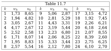
Consider the model relating the number of vacancies $w$ and the unemployment rate $u$

where $X_{k} = \ln w_{k}, h_{k} = \ln u_{k}, \varepsilon_{k} \sim \mathcal{N}\left(0 ; \sigma^{2}\right)$. Using the data from Table 11.7, find the OLS estimates of the parameters $\theta_{1}$ and $\theta_{2}$. Use the Durbin-Watson test to test the hypothesis $H_{0}: \rho = 0$ that the observation errors are uncorrelated, at the significance level $\alpha = 0,05$. If the hypothesis $H_{0}$ is rejected, assume that the sequence of random errors $\left\{ \varepsilon_{k}\right\}$ satisfies the first-order autoregression equation

where $e_{k}$ are centered Gaussian random variables with variance $\operatorname {Var}\left[e_{k}\right] = \sigma_{0}^{2}$. Find an estimate of the unknown coefficient $\rho$ in the autoregression equation.

Investigate the consumption function of Japan $X(h)$ over the period 1951-1962 for correlation of the observation errors. If the observation errors are correlated, find the realization of the GLS estimate of the vector of unknown parameters. Find an estimate of the covariance matrix of the error vector $E$. The data for the computations are given in Table 11.8 (data taken from: U. N. Yearbook of National Accounts Statistics, 1963). Here $X$ is aggregate individual consumption (trillion yen), and $h$ is aggregate personal income (trillion yen).

Table 11.8

Table 12.4 gives data on investment ($X$), government expenditure $\left(h_{1}\right)$, gross domestic product ($h_{2}$) and population $\left(h_{3}\right)$ for 28 countries in 1997. The quantities $X, h_{1}$ and $h_{2}$ are given in billions of US dollars, and $h_{3}$ in millions of people. Construct a dependence of the volume of investment on the volume of government expenditure and GDP of the form

where $\theta_{1}, \ldots , \theta_{4}$ are unknown parameters and $\varepsilon_{k} \sim \mathcal{N}\left(0 ; \sigma_{k}^{2}\right)$. Test the hypothesis $H_{0}: \sigma_{1}^{2} = \sigma_{2}^{2} = \cdots = \sigma_{28}^{2}$ using the Goldfeld-Quandt test at the significance level 0,05.

Table 12.4

Apply Bartlett's test to the data of Problem 1.

For the data of Problem 1, construct the dependence of investment on government expenditure and gross domestic product, dividing the values of all variables by the corresponding population value. Apply the Goldfeld-Quandt test to the new set of observations.

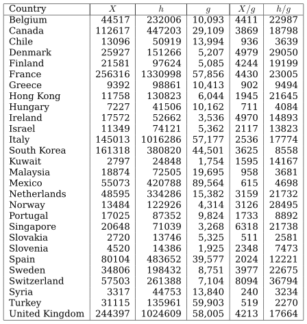
Investigate the dependence between manufacturing value added ($X$) and gross domestic product ($h$) on a sample of 28 countries for 1994 that includes both small and large countries (UNIDO Yearbook 1997). Table 12.5 gives the values of $X$ and $h$ in millions of US dollars, the population $(g)$ in millions of people, and the data in the last two columns in US dollars per person. Construct the OLS estimate of the parameters $\theta_{1}$ and $\theta_{2}$ for the model

Check for heteroscedasticity using one of the tests, assuming that the observation errors $\varepsilon_{k}, k = 1, \ldots , 28$ are uncorrelated and Gaussian. If heteroscedasticity is detected, eliminate it by dividing each observation by the population value. For this, the data from the last two columns of Table 12.5 can be used.

Table 12.5

Using a sample of 15 countries, estimate the parameters of the model $X = \theta_{1} + \theta_{2} h_{2}+\theta_{3} h_{3}$, where $X$ is per capita income; $h_{2}$ is the percentage of the labor force employed in agriculture; $h_{3}$ is the average level of education of persons over 25 years of age (the number of years spent in educational institutions). Test for the presence or absence of heteroscedasticity under the assumption that the observation errors are uncorrelated and have a Gaussian distribution; if it is detected, try to eliminate it.

Table 12.6

Derive formulas (13.11) - (13.13) for computing the mean-square error of an arbitrary estimate $\tilde{\theta }_{n}$ of the vector $\theta$.

Show that for an arbitrary ridge estimate $\bar{\theta }_{n}(k)$ the quantities $l_{n}(k)$ and $d_{n}(k)$ are determined by relations (13.16) and (13.17), respectively.

Show that for $k = 0$ we have $\bar{\theta }_{n}(k) = \widehat{\theta }_{n}, l_{n}(k) = 0, d_{n}(k) = \sigma^{2} \operatorname {tr}\left[W_{n}^{-1}\right]$.

Consider the limiting values of the ridge estimate $\bar{\theta }_{n}(k)$ and its characteristics $l_{n}(k), d_{n}(k)$ and $\Delta_{n}(k)$ as $k \rightarrow \infty$. What is the consequence of using too large values of the regularization parameter $k$ in the ridge estimation algorithm?

Table 13.1 gives the results of observations in a model with two parameters $\theta_{1}$ and $\theta_{2}$:

where $n = 10$, $\varepsilon_{m} \sim \mathcal{N}\left(0 ; 0,25\right)$, and the errors $\varepsilon_{m}$ and $\varepsilon_{i}$ are independent for $m \neq i$; the fourth column of Table 13.1 gives the exact values of the measured dependence $z_{m}^{(0)} = h_{1,m} \theta_{1}^{(0)}+h_{2,m} \theta_{2}^{(0)}$, where $\theta_{1}^{(0)}$ and $\theta_{2}^{(0)}$ are the true (unknown) values of the parameters $\theta_{1}$ and $\theta_{2}$.

Table 13.1

Using the data of Table 13.1, construct $\bar{\theta }_{n}(k)$ and $\Delta_{n}(k)$ for $k = 0,05$, $k = 0,5$ and $k = 5$. Choose the best of these estimates by the criterion of minimum mean-square error $\Delta_{n}(k)$.

Table 13.1 gives the results of observations in a model with two parameters $\theta_{1}$ and $\theta_{2}$:

where $n = 10$, $\varepsilon_{m} \sim \mathcal{N}\left(0 ; 0,25\right)$, and the errors $\varepsilon_{m}$ and $\varepsilon_{i}$ are independent for $m \neq i$; the fourth column of Table 13.1 gives the exact values of the measured dependence $z_{m}^{(0)} = h_{1,m} \theta_{1}^{(0)}+h_{2,m} \theta_{2}^{(0)}$, where $\theta_{1}^{(0)}$ and $\theta_{2}^{(0)}$ are the true (unknown) values of the parameters $\theta_{1}$ and $\theta_{2}$.

Table 13.1

Let $\tilde{\theta }_{n}$ equal $\widehat{\theta }_{n}$ or $\bar{\theta }_{n}(0,0167), \widetilde{z}_{m} = \widetilde{h}_{m} \widetilde{\theta }_{n}$ be the corresponding estimate of the exact value of the measured dependence $z_{m}^{(0)} = h_{m} \theta^{(0)}$, $m = 1, \ldots , n$. Let also $\delta_{n} = \sum_{m = 1}^{n}\left(\widetilde{z}_{m}-z_{m}^{(0)}\right)^{2}$. For which of the estimates will the quantity $\delta_{n}$ be smaller? Does the quantity $\delta_{n}$ change significantly when passing from the OLS estimate $\bar{\theta }_{n}(0)$ to the ridge estimate $\bar{\theta }_{n}(0,0167)$? Is the following statement true: least squares does not make it possible to construct ``good'' estimates of the parameters $\theta^{(0)}$, but does make it possible to estimate quite accurately the measured dependence $\left\{ z_{m}^{(0)}, m = 1, \ldots , n\right\}$?

Using the data from Table 13.3, find estimates of the parameters of the production function model $Y = F(K, L)$ if:

Using the data given in Table 14.1, estimate the average accrued wage in the Central Federal District by the methods of least squares and least absolute deviations. Analyze the data for anomalous values and reject them.

Consider the linear regression model

where $y_{k}$ is the per capita income in the $k$-th region of the Central Federal District, and $x_{k}$ is the average accrued wage in the same region (Table 14.2). Find estimates of the parameters $\theta_{1}$ and $\theta_{2}$ using the OLS and LAD algorithms.

Under the conditions of Example 14.3, analyze the data for outliers using the algorithm for rejecting anomalous data.

Using the data of Example 14.6, plot the estimates of the dependence $y(x) = \theta_{1}+\theta_{2} x$ for various types of parameter estimates. Construct forecast values of $y(x)$ at the points $x = 6 ; 6,5 ; 7$ and compare them with the exact values $y(x) = -1+2 x$ at these points. Analyze the effect of outliers on the accuracy of the obtained forecasts.

Table 14.4 gives the indices of output $Y_{k}$, capital inputs $K_{k}$ and labor inputs $L_{k}$ for $n = 10$ years (USA, 1913-1922).

Table 14.4

The relationship between these variables is assumed to have the form

Find estimates of the parameters $\theta_{1}$ and $\theta_{2}$ by OLS and LAD. Find a robust estimate of the parameter $\sigma^{2} = \operatorname {Var}\left[\varepsilon_{k}\right]$. Analyze the data for outliers and reject them.

Using the data of Table 15.4, estimate the parameters of the Cobb-Douglas production model [6] by the method of reducing the model to a linear one:

Table 15.4 (the data are given as percentages of the base year 1960, $i = 11$)

Using the data of Table 15.1, estimate the parameters of the model

Table 15.1

by the Gauss-Newton method. Compare with the results of Example 15.1.

Under the conditions of Example 15.2, find exact expressions for the components of the vector $F_{i}^{(m)}$.

The dependence of the variable $y$ on $x$ has the form of a rational function

Develop an algorithm for estimating the parameters $\left\{ \theta_{1}, \ldots , \theta_{4}\right\}^{\top }$ from the observations

by the Gauss-Newton method.

Let $g_{\alpha }(u) := u\left(\alpha - \; \mathbb {1}_{u < 0}\right)$, where $\alpha \in (0, 1)$. Show that $\mathbb {E}\left[g_{\alpha }\left(X-x_{\alpha }\right)\right]$ is a convex function of $x_{\alpha }$.

For the linear regression model $X_{k} = h_{k}^{\top }\theta +e_{k}$, consider the quantile regression problem $\widehat{\theta }(\alpha ) := \arg \min_{\theta } J_{\alpha }(\theta )$, where $J_{\alpha }(\theta ) := \sum_{k = 1}^{n} g_{\alpha }\left(X_{k}-h_{k}^{\top }\theta \right)$ and $g_{\alpha }(u) := u\left(\alpha - \; \mathbb {1}_{u < 0}\right)$. Show that the solutions of the problems in Examples 14.5 and 14.6 obtained by the variationally weighted least squares (VWLS) method coincide with the solutions of this quantile regression problem for $\alpha = 0,5$ constructed from the same observations.

For the simple regression model

where $\varepsilon_{k}$ are independent centered random variables with equal variance, solve the quantile regression problem $\widehat{\theta }(\alpha ) := \arg \min_{\theta } \sum_{k = 1}^{n} g_{\alpha }\left(X_{k}-\theta_{1}-\theta_{2} h_{k}\right)$ (where $g_{\alpha }(u) := u\left(\alpha - \; \mathbb {1}_{u < 0}\right)$) from the three observations $\left(h_{k}, X_{k}\right) = [(-1,-1) ;(0,2) ;(1 ; 0)]$ for various values of $\alpha \in (0,1)$. Analyze the results obtained, using Theorem 16.2.

For the observations described by the linear regression equation $X_{k} = \theta_{1}+\theta_{2} h_{k}+\varepsilon_{k}$, $k = 1, \ldots , n$, where $\varepsilon_{k} \sim \mathcal{N}\left(0 ; \sigma^{2}\right)$, given in Table 11.3, construct a plot showing the observations and the solution of the quantile regression problem $\widehat{\theta }(\alpha ) := \arg \min_{\theta } \sum_{k = 1}^{n} g_{\alpha }\left(X_{k}-\theta_{1}-\theta_{2} h_{k}\right)$ (where $g_{\alpha }(u) := u\left(\alpha - \; \mathbb {1}_{u < 0}\right)$) for $\alpha = [0,05,0,1, \ldots , 0,95]$.

Table 11.3