Simple Regression
[30/100%]This regression equation was estimated using data on college applicants who were admitted both to Pomona College and to another college ranked among the top 20 small liberal arts colleges by US News World Report:
where: fraction of students who were admitted to both this college and Pomona College who enrolled at Pomona college; average value X = US. News World Report ranking of this college () standard error
How were the numbers .2935 and .0293 obtained? (Do not show any formulas; explain in words the basis for the formulas.)
Explain why you are not surprised that the R-squared for this equation is not 1.0.
Does the coefficient of have a plausible value?
Is the estimated coefficient of statistically persuasive?
What is the null hypothesis in (d)?
What is the predicted value of for ?
Why should we not take the prediction in (f) seriously?
Explain why you either agree or disagree with each of these claims about the simple regression model:
If the estimated slope in a simple regression equation is negative, it cannot be statistically significant.
The estimated correlation coefficient doesn't depend on which variable is the dependent variable and which is the explanatory variable.
Ordinary least squares assumes that the explanatory variable is normally distributed.
Two researchers used annual data for 2000-2021 to estimate a simple regression model, where percentage change in the SP 500 from January 1 through January 31 and percentage change in the SP 500 index of stock prices from February 1 through December 31 of that same year:
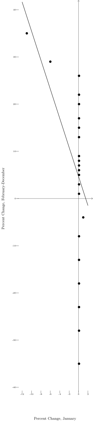
The authors reported that -value -value .1917. The beta is not substantial because the -value is less than 2. We can reject the null hypothesis. Our results show that FebruaryDecember change in the SP 500 does not depend on the change in January. Identify five distinct problems with this analysis.
The equation was estimated by ordinary least squares. Explain why you either agree or disagree with these statements:
Least squares regression minimizes the
is equal to the correlation coefficient squared.
A doubling of the number of observations, with the new data exactly replicating the original data, would increase .
means .
A researcher wanted to investigate burnout in competitive mountain biking. He looked at every California U23 (ages 19-22) mountain biker in 2012, and calculated the total number of sanctioned events they had competed in while in U23 and while they were in Junior racing (ages 17-18). The least squares regression was , with for the slope estimate and R -squared .
What are the most important problem(s) with these data?
Which variable in the regression equation should be the dependent variable?
Is the two-sided p-value for the slope estimated less than .05?
Explain why you either agree or disagree with this interpretation of the regression results: "This shows that racers generally raced close to the same number of times as a junior and as a U23."
A researcher specified this time-series model
where: annual percentage change in household spending annual percentage change in the SP 500 index of stock prices He reported these results
Estimate of
Estimate of > Estimate of > for test of :
What two mistakes do you see in these reported results?
Data were collected for 25 new cars on the car's weight and estimated highway miles per gallon . The model was estimated by ordinary least squares in three different ways: (a) the data were arranged alphabetically by car name; (b) the data were arranged numerically from the lightest car to the heaviest; and (c) the data were arranged numerically from the lowest miles per gallon to the highest. Which procedure yielded the smallest estimate of the intercept? Which yielded the highest estimate?
The equation was estimated by ordinary least squares. How would a doubling of the number of observations, with the new data exactly replicating the original data, affect the
estimates of the slope and intercept?
standard error of the estimate of the slope?
-value of the estimate of the slope?
?
A regression model was constructed to predict the sale price of homes in Elm City:
We looked at the list (asking) prices for 60 homes that are for sale in Elm City. We wrote down the square footage and price of the property and used that information to make a scatterplot with a line of least regression. The relationship between square footage and price of the listing was positive. The equation is , where square footage and list price. How would you improve this study and the report of the results?
Critically evaluate:
Many people believe that the 1979 spike in oil prices increased the unemployment rate in the United States. However, when I used monthly data for 1979 to estimate the equation , where is the unemployment rate and is the price of Texas crude oil, the estimated slope was not statistically significant-demonstrating that oil prices, in fact, had no effect on the unemployment rate.
A researcher used least squares to estimate the equation , where college GPA and high school GPA. First, he estimated the equation using all his data. Then, he separated his data into male and female students and estimated separate equations for each sex. Identify three apparent errors you see in these reported results.
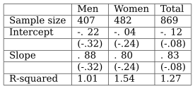
(): standard error
A 2005 linear regression estimated the relationship between the dollar prices P of 45 used 2001 Audi A4 2.8L sedans with manual transmissions and the number of miles M the car had been driven:
The standard errors are in parentheses.
Does the value 16,958 seem reasonable?
Does the value -.0677 seem reasonable?
Is the estimated relationship between M and P statistically persuasive?
Should the variables be reversed, with M on the left-hand side and P on the right-hand side?
Suppose that the true relationship is , where C is the car's condition (scale of , with 5 best) and , and are all positive. If and are negatively correlated, does the omission of from the estimated equation bias the estimate of upward or downward?
Here is an excerpt from a debate between two famous economists on the relationship between the growth of the money supply and the rate of inflation. Which economist do you agree with on the question of whether regression implies causation? Steve Hanke: I related the growth rate in the money supply to the inflation rate [in] 147 countries and the money supply measure I used is M2 and what do we end up with? We have almost a perfect correlation. John Cochrane: Correlation is not causation. We've known that forever. Steve Hanke: I also ran a regression and that does imply causation. John Cochrane: Oh, no no. Correlation does not imply causation. Come on now.
A researcher obtained the Scholastic Aptitude Test (X) scores and college grade point averages (Y) of 396 college students and reported these regression results:
(): std. devs. [ ]: t-values
There is a major error in these results. What is it?
The researcher concluded that, "Therefore I reject the null hypothesis and conclude that SAT scores and grades are not related." What is the basis for this conclusion and why is it wrong?
A study of 15 stocks that were wildly popular in the 1970s collected these data: (1) the December 1972 price earnings ratio (P/E) and (2) the annual percentage rate of return (R) from 1973 through 2000. What statistical test would you use to see if stocks with high P/E ratios tended to have low annual returns? (You do not have to actually do the test, just identify it clearly.) Be sure to identify the null hypothesis and how you would test it.
| 1972 P/E | R | ||
|---|---|---|---|
| Polaroid | 90.7 | -6.07 | |
| McDonald's | 85.7 | 11.85 | |
| Walt Disney | 81.6 | 10.58 | |
| Avon Products | 65.4 | 6.30 | |
| Kresge (now Kmart) | 54.3 | 1.20 | |
| Simplicity Pattern | 53.1 | -2.01 | |
| Xerox | 48.8 | -1.99 | |
| Eastman Kodak | 48.2 | 2.68 | |
| Coca-Cola | 47.6 | 14.64 | |
| IBM | 37.4 | 8.65 | |
| Procter \ | Gamble | 32.0 | 12.27 |
| PepsiCo | 29.3 | 16.17 | |
| General Electric | 26.1 | 16.85 | |
| Philip Morris | 25.9 | 18.00 | |
| Gillette | 25.9 | 14.89 |
A finance professor estimated this model to see if investors could increase their returns by buying stocks with high PEG ratios:
The model is
using these data for the 30 stocks in the Dow-Jones Industrial Average on December 31 of each year, during the period December 31, 2004, through December 31, 2021. > per share stock price on December 31 of that year > per share earnings during the preceding year > growth rate of earnings over the next 5 years > PEG = (P/E)/G > stock rate of return over next 7 months; January 1 through July 31
What are the two most important issues you would raise with this analysis?
Give at least three ways in which this presentation of the results could be improved:
| Coefficient | Standard Error | |
|---|---|---|
| Constant | .0198368 | .0238002 |
| PEG | .0017132 | |
| : Least squares estimates show a statistically significant relationship between PEG and R: |
**:
US taxpayers can either take a standard deduction or an itemized deduction based on property taxes, mortgage interest, charitable contributions, and a few other items. The deduction of property taxes and mortgage interest is intended to encourage home ownership which is thought to boost active citizenship, stable neighborhoods, and other positive externalities. A cross-section regression equation was estimated using 20152019 average values for each of the 58 counties in California: , where Y is the percentage of the eligible population who voted in the 2019 presidential primary election and X is the average value during the years 2015-2019 of the ratio of the number of homeowners divided by the total number of households in each county.
The estimated value of was 19.35 with a standard error of 20.95. Explain why you either agree or disagree with the authors' conclusion that
Although homeownership seems to have an economically significant and positive impact on voting percentage, statistical significance is lacking. Therefore, critics of the mortgage interest deduction have further support that home ownership does not encourage voting.
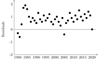
What is puzzling about this plot of the residuals from a least squares regression?
This regression equation was estimated using data for 481 California Census blocks that were more than Hispanic in 2008,
[97.12] [1.18] where: percentage of the two-party vote received by Barack Obama in the 2008 Presidential election X = median household income of Hispanics, $1000s of dollars The t -values are in brackets. Identify the logical error in this conclusion:
Income is not statistically significant; the -value is .27, meaning that there's a 27 chance we accept the null hypothesis that income has no effect on the Hispanic vote.
In 2005, Granite Construction applied for a permit to build a quarry near Temecula, California. Rocks would be dislodged from a mountain by daily blasts of 10,000 pounds of explosives and then crushed into gravel and sand that are used for concrete, asphalt, and other construction material. Mining and processing would go on 20 hours a day, 6 days a week, with 1,600 trucks entering and leaving the site daily.
The proposed quarry was in a mountain gap where ocean breezes carry cool air to the Temecula Valley. Residents were alarmed about the effect of this quarry on the city's economy and property values. However, an economist hired by Granite argued that in the city of Corona, which is 40 miles away and has had mines for many years, there was a "direct positive correlation" between annual mine production and property values over the past 20 years. Temecula residents evidently should be celebrating that their city was chosen for this quarry-which would have a positive effect on property values.
Provide a clear, persuasive refutation of this statistical argument.
A researcher used annual data for Major League Baseball (MLB) players for 1962 (when the current 162-game schedule was introduced) through 2011 to estimate this equation
where: average number of home runs per game that season X = average weight (in pounds) of MLB players and the standard errors are in parentheses. The average value of Y is 1.76 and the average value of X is 191.76.
Do you agree with the author's choice of which variable should be the dependent variable?
Why is the estimated intercept negative?
Is the estimated slope substantial, plausible, and statistically persuasive?
What fraction of the variation in is explained by ?
Critically evaluate:
The American Mustache Institute (AMI) is planning a "Million Mustache March" on the nation's capital. Their rallying cry: Pass the "Stimulus to Allow Critical Hair Expenses," or STACHE Act, which would "provide a annual tax deduction for expenditures on mustache grooming supplies." According to AMI research, mustached Americans earn 4.3 more money than "clean-shaven Americans" on average per year. Therefore incentivizing mustache growth would boost the economy. > "Given the clear link between the growing and maintenance of mustaches and income, it appears clear that mustache maintenance costs qualify for and should be considered as a deductible expense related to the production of income under Internal Revenue Code Section 212," wrote Dr. John Yeutter, a tax policy professor at Northeastern State University.
A researcher estimated a simple regression model using stock market returns for these pairs: return, average return 19301939; return, average return 1940-1949, and so on. The estimated correlation was positive, leading him to conclude that annual stock market returns could be used to predict returns over the next 10 years. What statistical flaw do you see in his procedure?
A study of the number of times that Trump tweeted the word economy each day and the daily high temperature in Moscow five days later found this relationship:
where: Moscow temperature daily Z-score for Trump tweets of the word economy The t -values are in brackets.
What is the average value of ?
What is the average value of Y?
Does the coefficient of Z seem statistically persuasive to you?
Does the coefficient of seem substantial to you?
Why are you deeply skeptical of this equation?
Explain why you either agree or disagree with these statements:
"Two variables with a +1.00 correlation move up and down at the same time, with the same magnitude."
"If the estimated slope in a simple regression model is larger than the true slope, then the estimated intercept is smaller than the true intercept."
Write the correct correlation value on each graph: :

A researcher estimated this equation for 74 breakfast cereals,
where: price per ounce X = grams of sugar per ounce
The t -values are in brackets. Explain why you either agree or disagree with this reasoning: "The Y-intercept of 0.3834 is statistically significant at the level. This result makes perfect sense because one would expect a box of cereal with zero grams of sugar to cost zero cents."
A study of the effect of driving speed on traffic fatalities estimated the following model by ordinary least squares,
where: deaths per million miles driven average speed, miles per hour The researcher used the data shown below:
| Year | ||
|---|---|---|
| 1980 | 57.0 | 1.6 |
| 1984 | 59.2 | 1.4 |
| 1985 | 59.5 | 1.3 |
The researcher argued that "supporters of lower speed limits would expect to be close to one, reflecting a strong, direct effect of X on Y." What is wrong with this argument?
Do you think that an ordinary least squares estimate of using these data will be positive or negative?
Why, no matter what the estimate of , are you suspicious of her data?
Least squares will be used to estimate the model , using annual data for 1991 through 2000. If and in 1991 and and in 2000, can the least squares estimate of possibly be negative? Explain your reasoning.
Least squares regression minimizes which of the following sums? Explain your reasoning.