Section 7.6

Positive Definite Matrices

[10/100%]
Show
LaTeX
Problem 7.6.1

Which of the following matrices are positive definite?

A=(1−1−1−151−115),B=(2068630808),C=(202062224). \mathbf{A} = \begin{pmatrix} 1 & -1 & -1 \\ -1 & 5 & 1 \\ -1 & 1 & 5 \end{pmatrix}, \quad \mathbf{B} = \begin{pmatrix} 20 & 6 & 8 \\ 6 & 3 & 0 \\ 8 & 0 & 8 \end{pmatrix}, \quad \mathbf{C} = \begin{pmatrix} 2 & 0 & 2 \\ 0 & 6 & 2 \\ 2 & 2 & 4 \end{pmatrix}.
?
Problem 7.6.2

Two masses m1m_1 and m2m_2 are suspended between three identical springs (with spring constant kk) as shown in Figure 7.6.7. Each mass is initially displaced from its equilibrium position by a horizontal distance and released to vibrate freely (assume there is no vertical displacement).
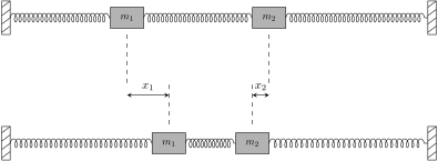
Figure 7.6.7Figure 7.6.7

?
(a)

If xi(t)x_i(t) denotes the horizontal displacement of mim_i from equilibrium at time tt, show that Mx→′′=Kx→\mathbf{M}\overrightarrow {x}'' = \mathbf{K}\overrightarrow {x}, where

M=(m100m2),x→=(x1(t)x2(t)),andK=k(2−1−12). \mathbf{M} = \begin{pmatrix} m_1 & 0 \\ 0 & m_2 \end{pmatrix}, \quad \overrightarrow {x} = \begin{pmatrix} x_1(t) \\ x_2(t) \end{pmatrix}, \quad \text{and} \quad \mathbf{K} = k\begin{pmatrix} 2 & -1 \\ -1 & 2 \end{pmatrix}.

(Consider a force directed to the left to be positive.) Notice that the mass-stiffness equation Mx→′′=Kx→\mathbf{M}\overrightarrow {x}'' = \mathbf{K}\overrightarrow {x} is the matrix version of Hooke's law F=kxF=kx, and K\mathbf{K} is positive definite.

(b)

Look for a solution of the form x→=eiθtv→\overrightarrow {x} = e^{i\theta t}\overrightarrow {v} for a constant vector v→\overrightarrow {v}, and show that this reduces the problem to solving an algebraic equation of the form Kv→=λMv→\mathbf{K}\overrightarrow {v} = \lambda \mathbf{M}\overrightarrow {v} (for λ=−θ2\lambda = -\theta^2). This is called a generalized eigenvalue problem because when M=I\mathbf{M} = \mathbf{I} we are back to the ordinary eigenvalue problem. The generalized eigenvalues λ1\lambda_1 and λ2\lambda_2 are the roots of the equation det⁡(K−λM)=0\operatorname {det}\left(\mathbf{K}-\lambda \mathbf{M}\right) = 0---find them when k=1k=1, m1=1m_1=1, and m2=2m_2=2, and describe the two modes of vibration.

(c)

Take m1=m2=mm_1 = m_2 = m, and apply the technique used in the vibrating beads example to determine the normal modes. Compare the results with those of part (b).

Problem 7.6.3

Three masses m1m_1, m2m_2, and m3m_3 are suspended on three identical springs (with spring constant kk) as shown below. Each mass is initially displaced from its equilibrium position by a vertical distance and then released to vibrate freely.
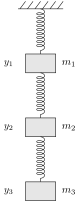
Three masses suspended in series by three identical springsThree masses suspended in series by three identical springs

?
(a)

If yi(t)y_i(t) denotes the displacement of mim_i from equilibrium at time tt, show that the mass-stiffness equation is My→′′=Ky→\mathbf{M}\overrightarrow {y}'' = \mathbf{K}\overrightarrow {y}, where

M=(m1000m2000m3),y→=(y1(t)y2(t)y3(t)),K=k(2−10−12−10−11) \mathbf{M} = \begin{pmatrix} m_1 & 0 & 0 \\ 0 & m_2 & 0 \\ 0 & 0 & m_3 \end{pmatrix}, \quad \overrightarrow {y} = \begin{pmatrix} y_1(t) \\ y_2(t) \\ y_3(t) \end{pmatrix}, \quad \mathbf{K} = k\begin{pmatrix} 2 & -1 & 0 \\ -1 & 2 & -1 \\ 0 & -1 & 1 \end{pmatrix}

(k33=1k_{33}=1 is not a mistake!).

(b)

Show that K\mathbf{K} is positive definite.

(c)

Find the normal modes when m1=m2=m3=mm_1=m_2=m_3=m.

Problem 7.6.4

By diagonalizing the quadratic form 13x2+10xy+13y213x^2+10xy+13y^2, show that the rotated graph of 13x2+10xy+13y2=7213x^2+10xy+13y^2=72 is an ellipse in standard form.

Figure 7.2.1 (p. 505) shows this ellipse: in the xyxy-coordinate system it is obliquely oriented, with the equation 13x2+10xy+13y2=7213x^2+10xy+13y^2=72; rotating the xyxy-coordinate system counterclockwise by 45∘45^{\circ } into a uvuv-coordinate system eliminates the cross-product term, and the ellipse's equation becomes u2/9+v2/4=1u^2/9+v^2/4=1.

?
Problem 7.6.5

Suppose that A\mathbf{A} is a real-symmetric matrix. Explain why the signs of the pivots in the LDU\mathbf{L}\mathbf{D}\mathbf{U} factorization for A\mathbf{A} reveal the inertia of A\mathbf{A}.

?
Problem 7.6.6

Consider the quadratic form

f(x→)=19(−2x12+7x22+4x32+4x1x2+16x1x3+20x2x3). f(\overrightarrow {x}) = \frac{1}{9}\bigl(-2x_1^2+7x_2^2+4x_3^2+4x_1x_2+16x_1x_3+20x_2x_3\bigr).
?
(a)

Find a symmetric matrix A\mathbf{A} so that f(x→)=x→TAx→f(\overrightarrow {x}) = \overrightarrow {x}^T\mathbf{A}\overrightarrow {x}.

(b)

Diagonalize the quadratic form using the LDLT\mathbf{L}\mathbf{D}\mathbf{L}^T factorization, and determine the inertia of A\mathbf{A}.

(c)

Is this a positive definite form?

(d)

Verify the inertia obtained above is correct by computing the eigenvalues of A\mathbf{A}.

(e)

Verify Sylvester's law of inertia by making up a congruence transformation C\mathbf{C} and then computing the inertia of CTAC\mathbf{C}^T\mathbf{A}\mathbf{C}.

Problem 7.6.7

Explain why each nonsingular A∈Cn×n\mathbf{A} \in \mathbb {C}^{n \times n} can be uniquely factored as A=RU\mathbf{A} = \mathbf{R}\mathbf{U}, where R\mathbf{R} is hermitian positive definite and U\mathbf{U} is unitary. This is the matrix analog of the polar form of a complex number z=reiθz = re^{i\theta }, r>0r>0, because 1×11\times 1 hermitian positive definite matrices are positive real numbers, and 1×11\times 1 unitary matrices are points on the unit circle.

?
Remark.
?

Hint: First explain why R=(AA∗)1/2\mathbf{R} = (\mathbf{A}\mathbf{A}^{*})^{1/2}.

Problem 7.6.8

Explain why trying to produce better approximations to the solution of the Dirichlet problem discretized as Lu→=g→\mathbf{L}\overrightarrow {u}=\overrightarrow {g} (the discrete Laplacian system of Example 7.6.2) by using finer meshes with more grid points results in an increasingly ill-conditioned linear system Lu→=g→\mathbf{L}\overrightarrow {u}=\overrightarrow {g}.

Example 7.6.2's discretization gives the eigenvalues of the discrete Laplacian L\mathbf{L} as λij=4−2cos⁡(iπn+1)−2cos⁡(jπn+1)\lambda_{ij} = 4 - 2\cos \bigl(\frac{i\pi }{n+1}\bigr) - 2\cos \bigl(\frac{j\pi }{n+1}\bigr) for i,j=1,2,…,ni,j = 1, 2, \ldots , n, where nn is the number of interior grid points per side.

?
Problem 7.6.9

For a given function ff the equation ∇2u=f\nabla^2 u = f is called Poisson's equation. Consider Poisson's equation on a square in two dimensions with Dirichlet boundary conditions. That is,

∂2u∂x2+∂2u∂y2=f(x,y)withu(x,y)=g(x,y) on the boundary. \frac{\partial ^2 u}{\partial x^2} + \frac{\partial ^2 u}{\partial y^2} = f(x,y) \quad \text{with} \quad u(x,y) = g(x,y) \text{ on the boundary.}

Discretize the problem by overlaying the square with a regular mesh containing n2n^2 interior points at equally spaced intervals of length hh, as in Example 7.6.2. Let fij=f(xi,yj)f_{ij} = f(x_i,y_j), and define f→\overrightarrow {f} to be the vector f→=(f11,f12,…,f1n∣f21,f22,…,f2n∣⋯∣fn1,fn2,…,fnn)T\overrightarrow {f} = (f_{11}, f_{12}, \ldots , f_{1n} \mid f_{21}, f_{22}, \ldots , f_{2n} \mid \cdots \mid f_{n1}, f_{n2}, \ldots , f_{nn})^T. Show that the discretization of Poisson's equation produces a system of linear equations of the form Lu→=g→−h2f→\mathbf{L}\overrightarrow {u} = \overrightarrow {g}-h^2\overrightarrow {f}, where L\mathbf{L} is the discrete Laplacian and where u→\overrightarrow {u} and g→\overrightarrow {g} are as described in Example 7.6.2.

?
Problem 7.6.10

As defined in Exercise 5.8.15 and discussed in Exercise 7.8.11, the Kronecker product (sometimes called tensor product, or direct product) of matrices Am×n\mathbf{A}_{m \times n} and Bp×q\mathbf{B}_{p \times q} is the mp×nqmp \times nq matrix

A⊗B=(a11Ba12B⋯a1nBa21Ba22B⋯a2nB⋮⋮⋱⋮am1Bam2B⋯amnB). \mathbf{A} \otimes \mathbf{B} = \begin{pmatrix} a_{11}\mathbf{B} & a_{12}\mathbf{B} & \cdots & a_{1n}\mathbf{B} \\ a_{21}\mathbf{B} & a_{22}\mathbf{B} & \cdots & a_{2n}\mathbf{B} \\ \vdots & \vdots & \ddots & \vdots \\ a_{m1}\mathbf{B} & a_{m2}\mathbf{B} & \cdots & a_{mn}\mathbf{B} \end{pmatrix}.

Verify that if In\mathbf{I}_n is the n×nn\times n identity matrix, and if

An=(2−1−12−1⋱⋱⋱−12−1−12)n×n \mathbf{A}_n = \begin{pmatrix} 2 & -1 & & \\ -1 & 2 & -1 & \\ & \ddots & \ddots & \ddots \\ & & -1 & 2 & -1 \\ & & & -1 & 2 \end{pmatrix}_{n \times n}

is the nnth-order finite difference matrix, then the discrete Laplacian is given by

Ln2×n2=(In⊗An)+(An⊗In). \mathbf{L}_{n^2 \times n^2} = (\mathbf{I}_n \otimes \mathbf{A}_n) + (\mathbf{A}_n \otimes \mathbf{I}_n).

Thus we have an elegant matrix connection between the finite difference approximations of the one-dimensional and two-dimensional Laplacians. This formula leads to a simple alternate derivation of (7.6.8)---see Exercise 7.8.12. As you might guess, the discrete three-dimensional Laplacian is

Ln3×n3=(In⊗In⊗An)+(In⊗An⊗In)+(An⊗In⊗In). \mathbf{L}_{n^3 \times n^3} = (\mathbf{I}_n \otimes \mathbf{I}_n \otimes \mathbf{A}_n) + (\mathbf{I}_n \otimes \mathbf{A}_n \otimes \mathbf{I}_n) + (\mathbf{A}_n \otimes \mathbf{I}_n \otimes \mathbf{I}_n).
?