AR-, MA-, and ARMA-models
[15/0%]Suppose that an AR(1)-process, , has the covariance function . Which AR(1)-process is it? What is the variance of the innovations?
Find the spectral density, , and the covariance function, , at time lag zero, one and two, of the AR(2)-process
where is a white innovation process with variance .
The covariance function of a signal, , in discrete time, has been well estimated at a few time lags:
We decide to use the following AR(2)-process to model the signal,
Find the innovation variance, the second AR-parameter, and the covariance function at time lag two.
The MA(q)-process
where is a white innovation process with unit variance, has covariance function , , , and , . Determine the order of the process, the MA-coefficients, and the spectral density.
Let , be independent random variables with expectation and variance . Define, for a constant ,
Choose , such that is an MA(3)-process. Determine the expectation, covariance function, and spectral density of .
Find expectation, covariance function, and spectral density of .
Let be a stationary AR(1)-process,
and let be an MA(2)-process,
where and are independent white Gaussian processes with unit variance. Realizations and estimated covariance functions of and are shown in Figure 7.13, but which subplot shows what?
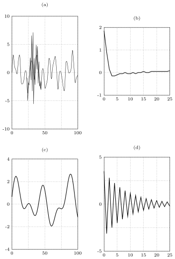 Figure 7.13 Realizations and estimated covariance functions of one AR(1)- and one MA(2)-process in Exercise 7:6.
Combine, in Figure 7.14, realizations, covariance functions, and spectral densities for two stationary processes.
 Figure 7.14 Realizations, covariance functions, and spectral densities to Exercise 7:7a.
Combine the processes with the correct pole-zero plot in Figure 7.15, where 'x' depicts poles and 'o' zeros. The processes are of the type AR or MA. State the type and order of the processes.
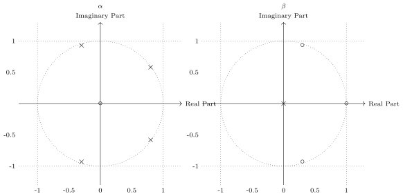 Figure 7.15 Pole-zero plots to Exercise 7:7b.
Figure 7.16 shows pole-zero plots, spectral densities, and covariance functions for three AR(2)-processes. Determine which figures that describe the same process.
 Figure 7.16 Pole-zero plots, covariance functions, and spectral densities of two processes in Exercise 7:8.
(This is a classical example of time series analysis in hydrology.) The Wabash river water level, (meter), is measured once every month. The following AR-type model has been suggested:
where is a white noise process with variance 4. What is the expected water level according to this model? What is the standard deviation?
Let be an AR(1)-process, , with . Construct a new process, , by using every second element of , that is: . Prove that is an AR(1)-process and that it thus can be written in the following form:
Also, compute and .
Compute the cross-covariance, , , where is an AR(1)-process: , and .
A random process, , is generated by filtering white noise:
where and are unknown. A simulation gives the following values:
Estimate and , using the given observations.
Use your estimates in (a) to estimate and .
Let be stationary with mean value and assume
where is Gaussian white noise with mean value zero and unit variance. The following values of are observed:
Estimate and compute a 95 confidence interval for your estimate.
Find the best one-step ahead predictor of the ARMA(1,1)-process defined by .
Figure 7.17 shows the mean wave height, , outside the Pakistan coast, as measured by a satellite passing the Indian Ocean on May 21, 1993. The process is well described by an AR(3)-model:
where is white noise with unit variance. Compute and from the first four covariances:
 Figure 7.17 Wave height, spectrum, and covariance function estimated using data, and spectrum and covariance function of the model in Exercise 7:15.