Interpreting multiple regression output tables
[9/100%]This multiple regression equation was estimated using 2005 data for 100 homes in Plano, Texas: where: home price square feet of living area G = garage square feet A = age of house in years BR = number of bedrooms BA = number of bathrooms if it has central air, 0 if not and standard errors are in parentheses.
Which of the estimated coefficients are statistically persuasive?
Provide a logical explanation for why the coefficient of BR might be negative.
Do you think that the coefficients in housing regression equations change over time? Why or why not?
A student estimated a regression model that used the number of pages in best-selling hardcover books to predict their prices. Explain why this conclusion is wrong: "The 0.75 R-squared is pretty large, when you consider that the price of a book is and of the price is explained by the number of pages."
The following multiple regression model was used to explain the sale prices (in thousands of dollars) for 60 single-family homes in Oxnard, California:
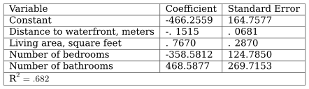
Interpret the -. 1515 coefficient.
Which coefficient estimates (other than the constant) are statistically persuasive?
Explain why you either agree or disagree with this argument: "The bedroom coefficient is negative because if the living area is fixed, doubling the number of bedrooms halves the size of each."
Explain why you either agree or disagree with this argument: "The bathroom coefficient is positive because homes with more bathrooms tend to be larger than homes with fewer bathrooms."
A study of home prices in a suburban Rhode Island town used these variables in a multiple regression model: price square feet number of bedrooms number of bathrooms Walk Score, a rating (from 0 to 100) for a given address, based on the walking distance from that address to a variety of key amenities. A Walk Score of 70 or above is generally considered good.
What is wrong with this interpretation of the results: "The coefficient of is negative because large homes that have high prices are usually secluded from grocery stores, coffee shops, and other desirable destinations."
Identify two ways in which this report of the estimation of a multiple regression equation could be improved:
| Variable | t-statistic | p-value |
|---|---|---|
| Variable1 | 2.47 | .02 |
| Variable2 | 1.70 | .09 |
| Variable3 | 6.31 |
How would you respond to this question?
I have run into a problem with missing values in my data. Some of the variables including GPA and parents' education have a lot of missing values. If I discard those individuals with missing values, then the dataset becomes very small, but if I replace all the missing values with zeros, the total sample size is about 35,000 and I am able to get statistically significant results.
A multiple regression model was used to estimate the relationship between a Major League Baseball (MLB) player's salary and his batting average and home runs:
| Mean | Standard Deviation | |
|---|---|---|
| S = annual salary, millions of dollars | 2.5 | 3.5 |
| B = batting average for season | . 263 | . 032 |
| number of home runs in season | 12.5 | 10.4 |

Can we conclude from these results that salaries are affected more by batting average than by home runs, or vice versa? Explain your reasoning.
Data for the top 100 money winners on the 1993 Professional Golf Association (PGA) tour were used to estimate the following equation:
| {} | {} | {} | {} | {} | {} |
where: Y = dollars won D = average length of drives from the tee, yards A = driving accuracy (percent of drives landing in fairway) G = percent of greens that were reached in par minus two strokes percent of those greens reached in par minus two that required only one putt percent of times player made par after hitting into sand The standard errors are in parentheses; the t -values are in brackets; and .
Which of the explanatory-variable coefficient are statistically significant at the level?
Which, if any, of the estimated explanatory-variable coefficients have plausible signs?
How can the intercept be negative if Y cannot be negative?
Does the fact that the coefficient of P is larger than the coefficient of D imply that, other things being equal, a player who is a good putter will win more money than a person who hits long drives? Explain.
Does the fact that the t -value for the coefficient of D is larger than the t -value for the coefficient of S imply that, other things being equal, a player who hits long drives will win more money than a person who is better at making par out of sand traps? Explain.
Do you agree or disagree with the following statements?
If R-squared is not high enough, you should add more explanatory variables.
If there is a multicollinearity problem, you should drop some explanatory variables.
If the null hypothesis is true, the p-value is more likely to be less than .10 than less than .05.
The least squares line goes through the sample means of X and Y.
The probability of A or B is equal to the probability of A plus the probability of .